Introduction
JANet Description
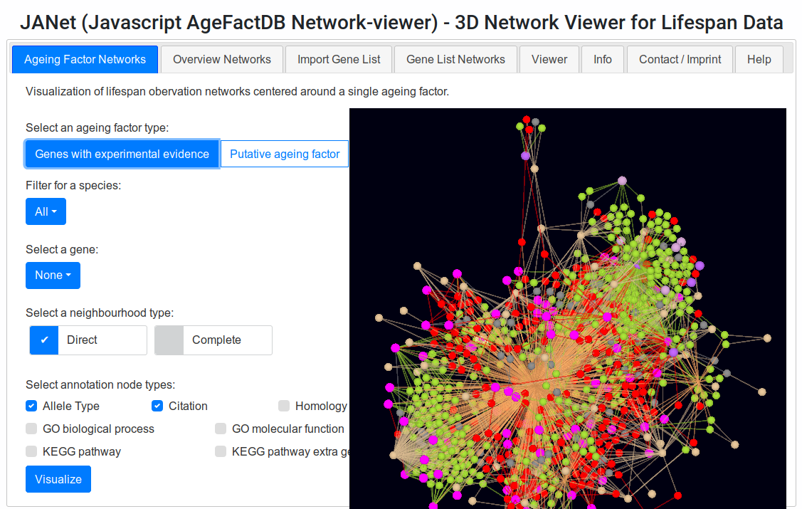
JANet (Javascript AgeFactDB Network-viewer) is a specialized 3D network viewer for Exploration and Visualization of ageing-related network data from AgeFactDB.
 JANet Web Browser Interface.
Screenshot of the JANet interface, menu combined with viewer .
JANet Web Browser Interface.
Screenshot of the JANet interface, menu combined with viewer .
Selected Features
- Interactive 3D network visualization
- 2D representation
- Stereo representation
- Ageing-related network data (AgeFactDB)
- Lifespan observations
- Ageing factors
- Augmentation nodes
- Augmentation with external domain knowledge
- Gene Ontology (GO)
- KEGG Pathways
- Genes of interest analysis
Requirements
- 4 GB main memory
- Modern Web browser with activated Javascript
Recommended:
- 16 GB main memory
- 64-bit system
- Modern web browser with activated Javascript
Availability
The application can be started from the server at http://sysbio.uni-ulm.de/software/janet
Source Code
The complete source code is available at http://sysbio.uni-ulm.de/software/janet/latest.zip
AgeFactDB
Description
AgeFactDB (http://agefactdb.jenage.de) is a database designed for the collection and integration
of ageing phenotype data including lifespan information.
Ageing factors are considered to be genes, chemical compounds or other factors such as dietary restriction, whose action results
in a changed lifespan or another ageing phenotype.
Any information related to the effects of ageing factors is called an observation and is presented on observation pages. To provide concise access to the complete information for a particular ageing factor, corresponding observations are also summarized on ageing factor pages.
In a first step, ageing-related data were primarily taken from existing databases such as the Ageing Gene Database--GenAge,
the Lifespan Observations Database and the Dietary Restriction Gene Database--GenDR. In addition, it was started to include
new ageing-related information.
Based on homology data taken from the HomoloGene Database, AgeFactDB also provides observation and ageing factor pages of genes
that are homologous to known ageing-related genes. These homologues are considered as candidate or putative ageing-related genes.
Ageing Factors
Currently there are implemented three types of ageing factors: Gene, Chemical Compound, and Other Ageing Factor.
Gene
If available, the NCBI Gene ID is used for the identification of genes, to avoid duplicate entries with different names.
If it is not provided, it is tried to assign it automatically using the synonym database GPSDB and the NCBI Gene database.
If multiple NCBI Gene IDs might match, no NCBI Gene ID is assigned and only gene symbol and species are used for the integration
Internally always gene symbol, species, and NCBI Gene ID are used to identify a gene. Depending on the information provided by
the data source, GPSDB, and NCBI Gene it is possible that the same gene symbol/species combination is included multiple times into AgeFactDB,
with and without one or more different NCBI Gene IDs.
Chemical Compound
Chemical compounds are currently identified by the name who was used in the AgeFactDB source databases. No synonym information is used yet within AgeFactDB.
Other Factor
Other factors are for example dietary restriction and heat shock.
Similar to chemical compounds they are currently only identified by their name. Because it is difficult to judge the slight differences
that might be involved for example between 'dietary restriction' and 'caloric restriction', it wasn't done any unification yet.
Putative Ageing Factors
In addition to genes with experimental ageing relevance evidence, AgeFactDB includes also genes homologous to these genes as putative ageing factors.
They are identified by a homology analysis based on the HomoloGene database from the NCBI.
In contrast to other ageing-related databases, where homologous genes are just named inside a gene page, they are included in the same way as
the genes with experimental ageing relevance evidence. This way the full features are also available for the putative ageing factors.
Ageing factors are discriminated from putative ageing factors inside the AgeFactDB web interface by a color coding system shown in the Figure below. Green indicates experimental evidence with an effect on ageing, red indicates
experimental evidence with no effect on ageing, and blue indicates computational ageing relevance evidence. The color of all observations
assigned to an ageing factor determine the color of the ageing factor, with the following priority: green, red, blue. In addition to the
major color, all other assigned colors are also indicated as small squares.
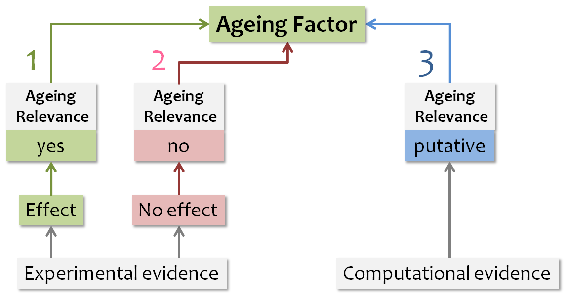 Ageing Relevance Evidence Color Codes.
Color coding system to indicate the type of ageing relevance evidence available for ageing factors.
Ageing Relevance Evidence Color Codes.
Color coding system to indicate the type of ageing relevance evidence available for ageing factors.
The priority for assigning a color to the ageing factor is indicated by the number:
- Highest priority – 1
- Lowest priority – 3
Observations
Currently there are implemented three types of observations:
- Ageing Phenotype Data Type 1
- Ageing Phenotype Data Type 2
- Homology Analysis
The names are the 'official' names used in the web interface. Initially, the first two types were named 'phenotype' and 'lifespan'.
But this didn't really fit, because lifespan is also a phenotype and because some phenotype observations also contained lifespan data.
So it was switched to a technical distinction:
- Data Type 1 - free-text ageing phenotype observations
- Data Type 2 - structured ageing phenotype observations
- Homology analysis - structured computational observations.
Unification
The same genes might have been integrated into two different source databases or even the same source database with different names.
It was tried to resolve this by using the gene/protein synonym database GPSDB and integrate the gene into AgeFactDB using the name
marked as preferred name in GPSDB.
All name changes are listed in a table within the release page.
A partial list of the ageing factor name changes as a result of the unification is shown below:
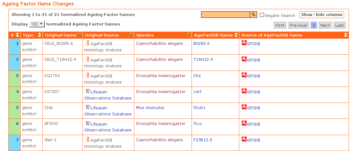 Unification of Ageing Factor Names.
Extract from the AgeFactDB release page table showing changes in ageing factor names during the import from other databases.
Unification of Ageing Factor Names.
Extract from the AgeFactDB release page table showing changes in ageing factor names during the import from other databases.
Network Data
The lifespan observation data from AgeFactDB was transformed into a network data representation.
Lifespan Observation/Ageing Factor Nodes
Each lifespan observation (LO) and each ageing factor (AF) is represented by a network node. Ageing factors involved in a specific lifespan observation are each linked to it by an edge. This facilitates to understand the often very complex system of observations involving overlapping sets of ageing factors at different conditions.
Annotation Nodes
Cruical annotation data is not just attached to an observation or ageing factor, visible for example while hovering a node. Instead it expands the network as annotation node (ANN).
AgeFactDB Annotation Nodes
JANet currently supports the following types of annotation nodes from AgeFactDB data:
- Allele Type (AT)
- Citation (CI)
- Species (SP)
Expert Knowledge Annotation Nodes
In addition to AgeFactDB-based annotation nodes, JANet also supports annotation nodes based on expert knowledge from other databases:
- Gene Ontology(GO)
- KEGG Metabolic Pathways (extracted from the BioSystems database)
Network Layout Algorithms
3D network visualization requires to define a position in the three-dimensional space for each node, called a network layout.
Spring-force algorithms provide often useful layouts. In these algorithms connected nodes attract each other and unconnected nodes repel each other.
The attracting and repelling forces are calculated like for spring forces in physics. As a start, the nodes are usually placed on random positions. The
forces are then calculated for each node pair in an iterative process to define new node positions, until an equilibrium is reached or a fixed number
of iterations.
3D-forced
JANet uses the 3D-forced-layout algorithm as default.It is implemented in Javascript and uses a velocity Verlet numerical integrator to calculate the node positions.
It generates good layouts for medium sized networks, up to a few hundred nodes.
Fruchterman-Reingold
JANet uses the Fruchterman-Reingold algorithm in an adapted version for 3D layout, implemented in Javascript.
It generates good layouts for small sized networks, up to about hundred nodes.
FMMM - Fast Multipole Multilevel Method
For larger networks the FMMM (Fast Multipole Multilevel Method) algorithm used in BioLayout Express 3D, another 3D network viewer, provides
better layouts than the Fruchterman-Reingold algorithm. It is not implemented in JANet directly yet. Instead, JANet uses
an adapted BioLayout Express 3D version as an automatic server-sided external layout generation tool for larger networks. FMMM layouts are cached on the server.
Visualization Techniques
JANet provides several visualization techniques for lifespan observation (LO) networks of ageing factors (AFs).
Node color and size are used there
to speed-up the lookup of node properties by visual perception for all nodes at once. Generally these properties are the node type and the qualitative
and quantitative lifespan change.
The edge color is usually inherited from the node of a pair whose color carries specific information for the other
node. For AF/LO edges this is the LO node, whose color usually indicates the direction of the lifespan change (increased, decreasd, none).
Direct Neighbourhood
The direct neighbourhood network provides a compact view that is focused on a single AF. It shows LOs in which this AF (AF1) was manipulated and all additional AFs (AF2 and AF3).
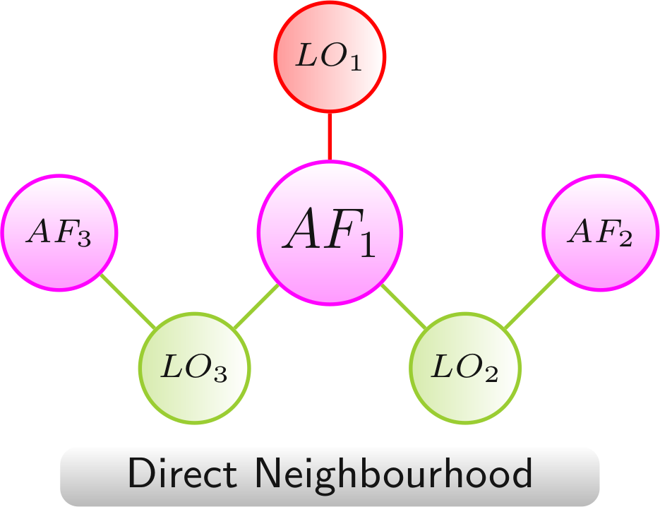
Color scheme:
AF,
LO - increased lifespan,
LO - decreased lifespan
Complete Neighbourhood
The complete neighbourhood links a central AF(AF1) with all AFs (AF2 - AF5) and LOs (LO1 - LO8) that can be reached via sequences of LOs and AFs.
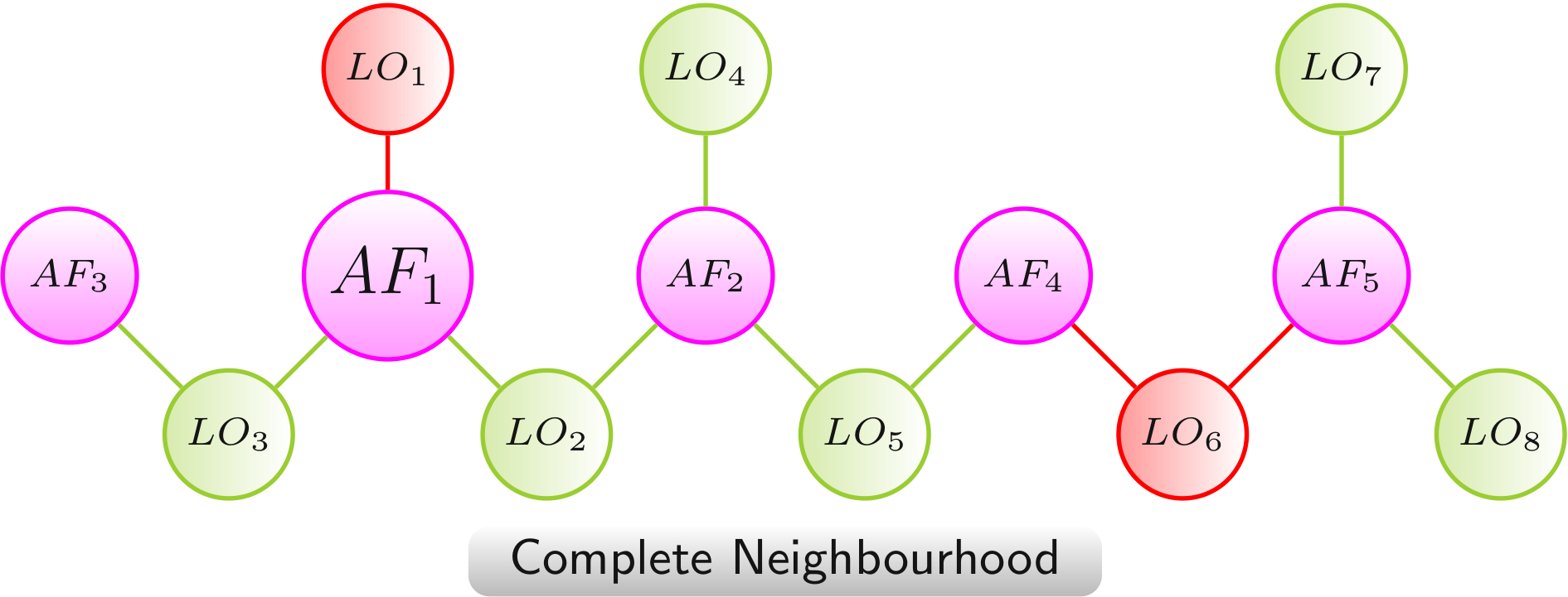
Color scheme:
AF,
LO - increased lifespan,
LO - decreased lifespan
Augmentation via Annotation Nodes
The augmented network provides additional information on AFs and / or LOs as annotation nodes. Additional information enables more complex queries and leads to a semantic clustering of AFs and / or LOs in the network layout.
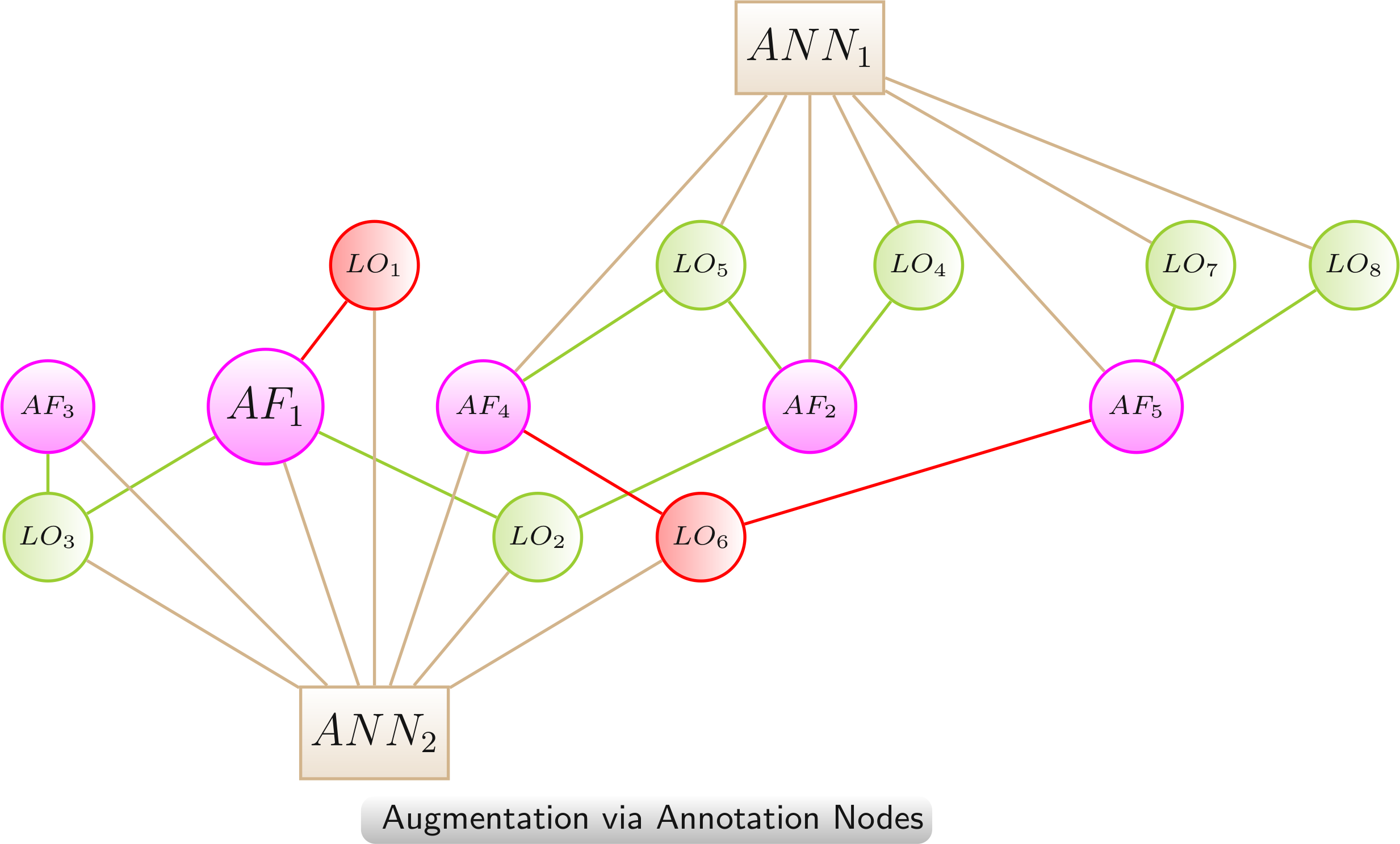
Color scheme:
AF,
LO - increased lifespan,
LO - decreased lifespan,
annotation
Data Transfer betwen Nodes
Data transfer between nodes is used for reducing complexity. Information from removed / hidden nodes is visualized by a change of color. AFs gain LO-colors.
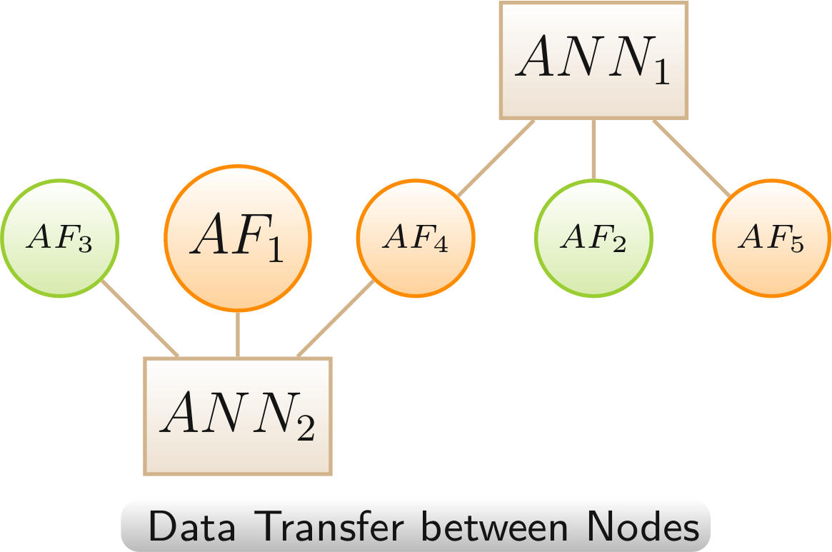
Color scheme:
annotation,
AF - linked only to LOs with increased lifespan,,
AF - linked to LOs with highly mixed lifespan changes (increased and decreased > 20%)
Multispecies Technique
Chemical compounds and Other factor AFs can be linked to LOs of multiple species. Species nodes (SP) are linked to corresponding LOs. Links between the AFs and the species nodes are left out for a clearer network view. The layout algorithms group the network according to the involved organisms.
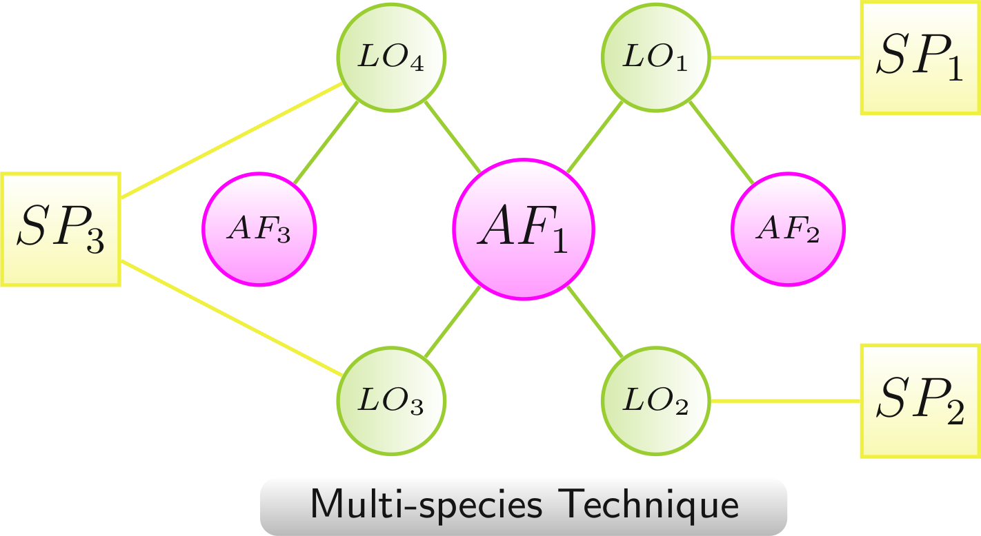
- AF1 to SP1 via LO1, to SP2 via LO2, and to SP3 via LO3 and LO4
- AF2 to SP1 via LO1
- AF3 to SP3 via LO4
Color scheme:
AF,
LO - increased lifespan,
LO - decreased lifespan,
species
JANet Web Browser Interface
Overview
JANet has a modern web browser interface with eight tabs:
- Ageing Factor Networks
- Overview Networks
- Import Gene List
- Gene List Networks
- Viewer
- Info
- Contact / Imprint
- Help
Tabs
Ageing Factor Networks
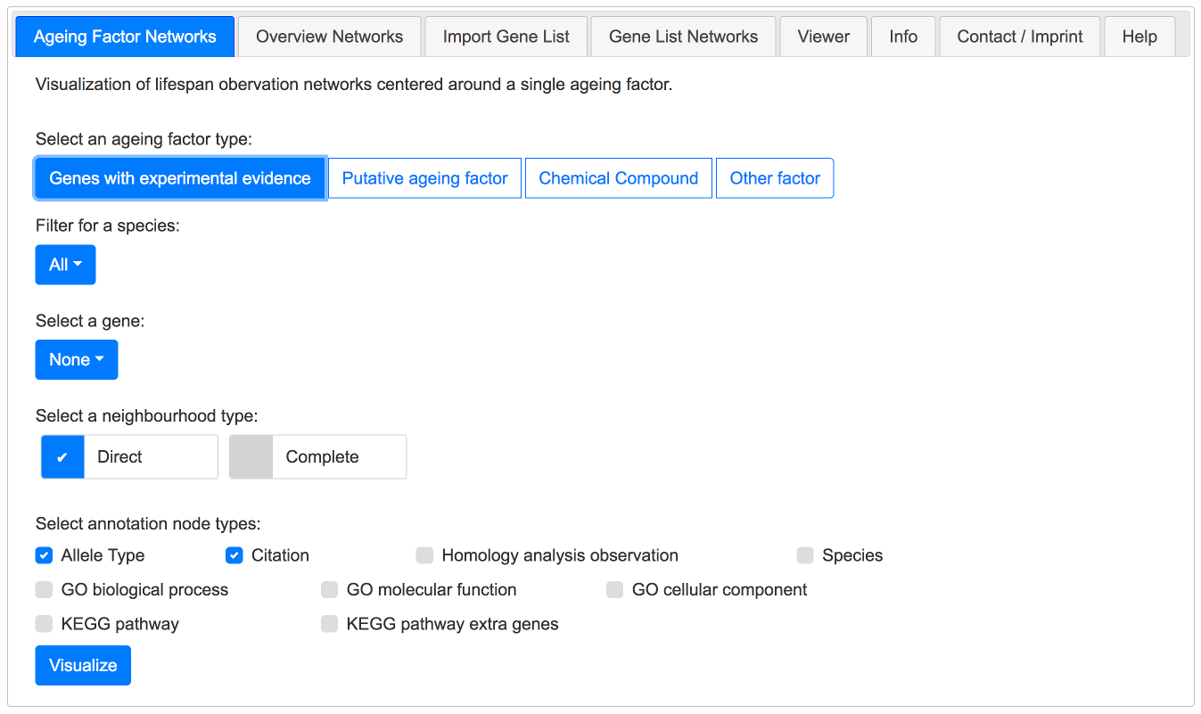 Ageing Factor Networks Tab
This tab can be used to choose a specific ageing factor along with it's annotation nodes. First you select an ageing factor type. Next you can filter for a species. Then you select an ageing factor. By default the direct neighbourhood of the ageing factor is selected. The complete neighbourhood can be used as well.
By visualizing the network (Button Visualize) the Viewer is activated and the network is shown.
Overview Networks
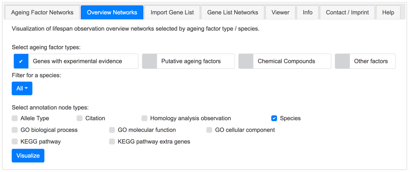 Overview Networks Tab
To get an overview of a set of ageing factors, this tab can be used to visualize these. A filter for species and a selection of annotation nodes can be choosen.
Import Gene List
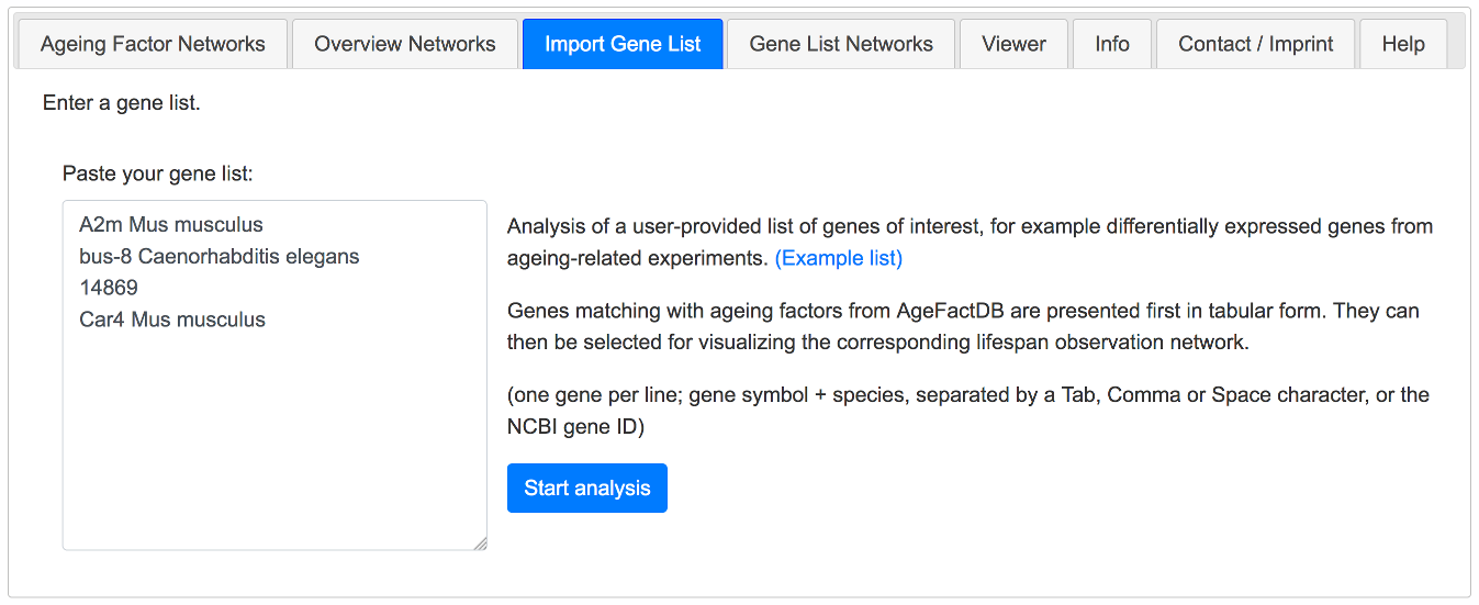 Import Gene List Tab
If you want to analyse a specific gene set, you can upload your gene list to JANet and use the third tab to import your data and start the analysis.
The list could contain for example differentially expressed genes from an ageing-related experiment.
Gene List Networks
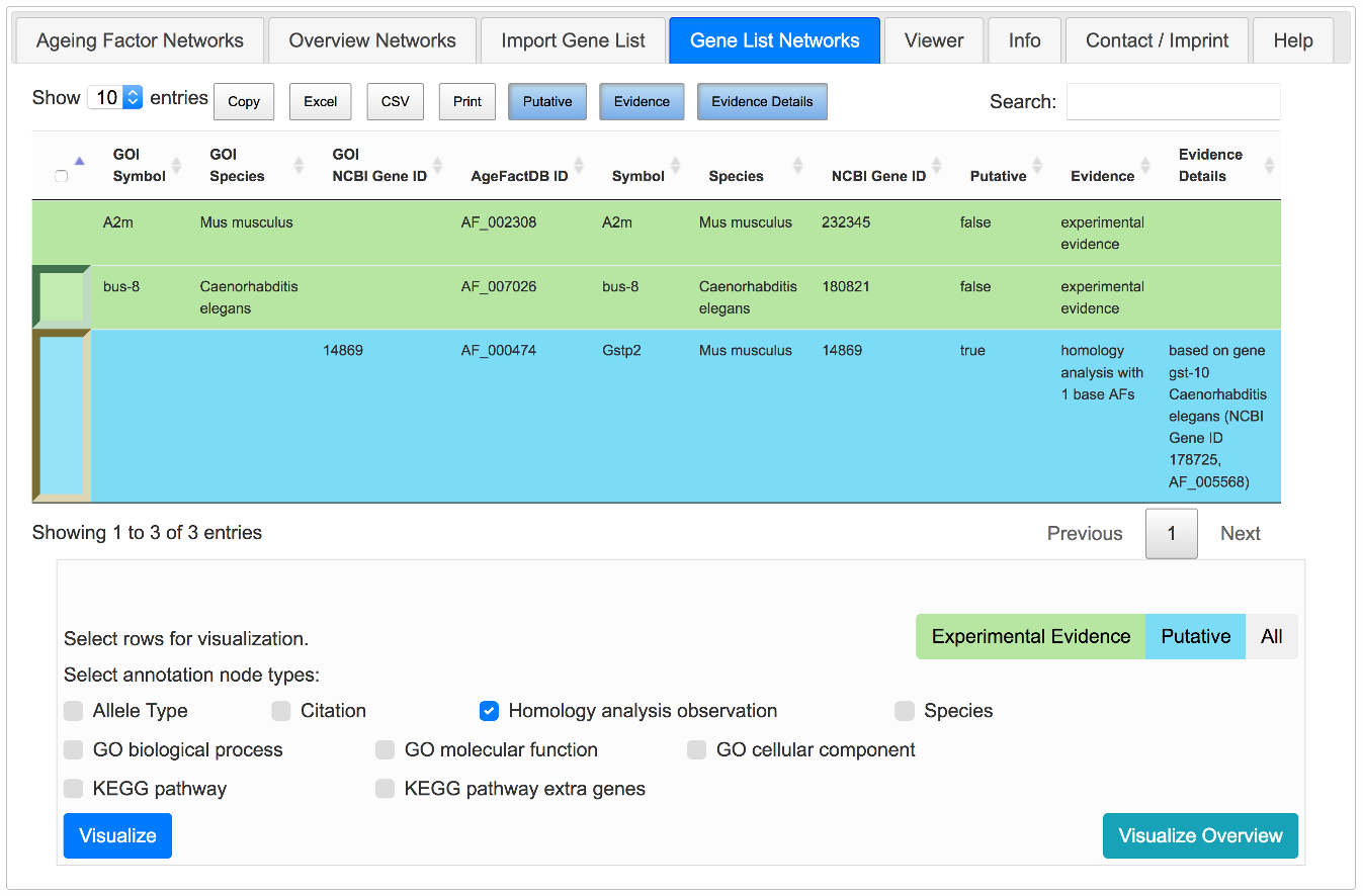 Gene List Networks Tab
Genes matching with ageing factors from AgeFactDB are presented in tabular form. You can then select genes of interest for visualizing the corresponding lifespan observation network or get an overview network of all found genes of interest.
This overview network has some special characteristics compared to the standard overview networks:
- Only matching ageing factors / putative ageing factors are included to provide a clearer overview
- Genes from the gene list are marked by a halo
- All ageing factor labels are displayed initially
- FMMM layout recommended, because it provides a tiled layout of unconnected subnetworks
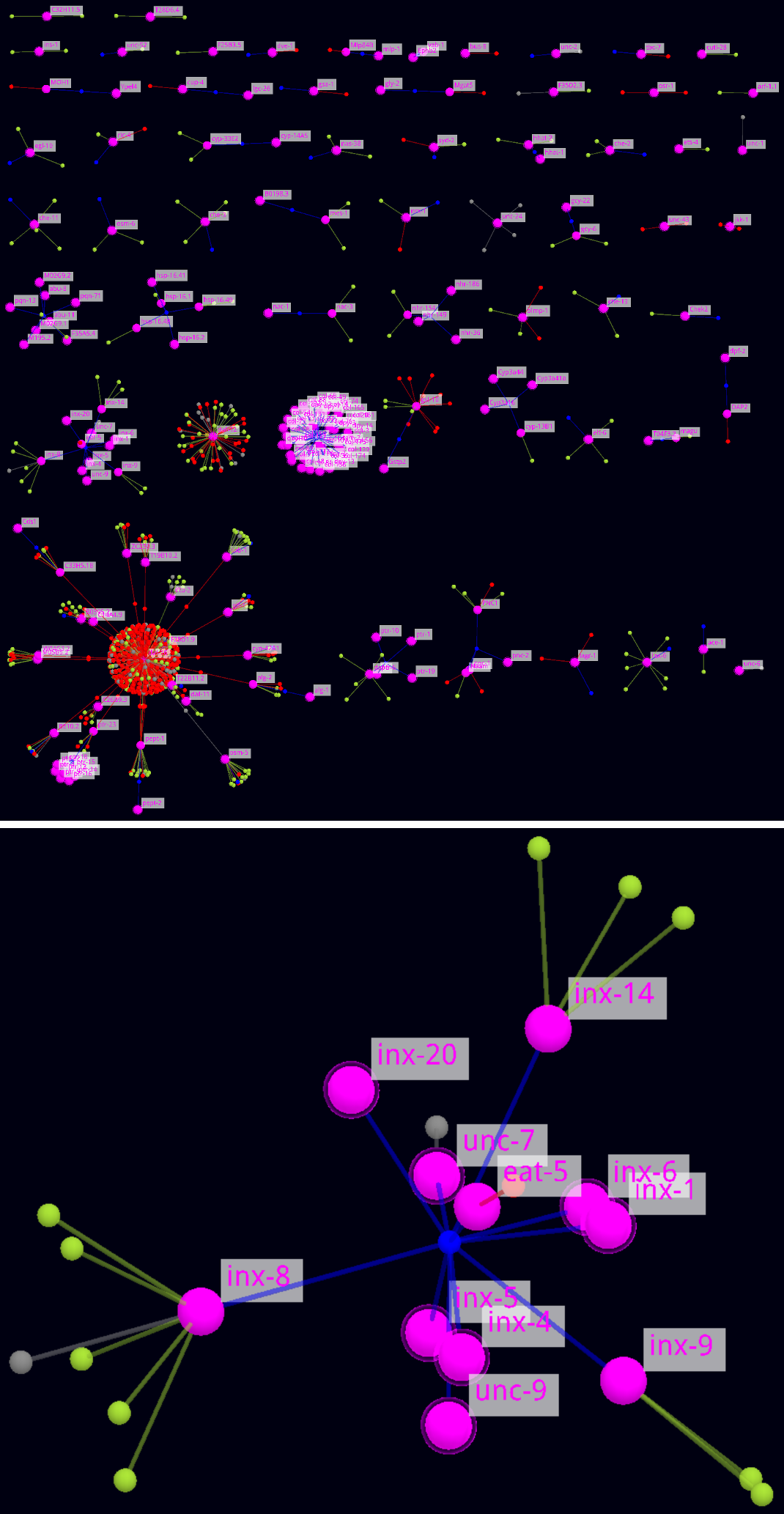 Example - Gene List Networks Overview (complete + zoomed part)
Viewer
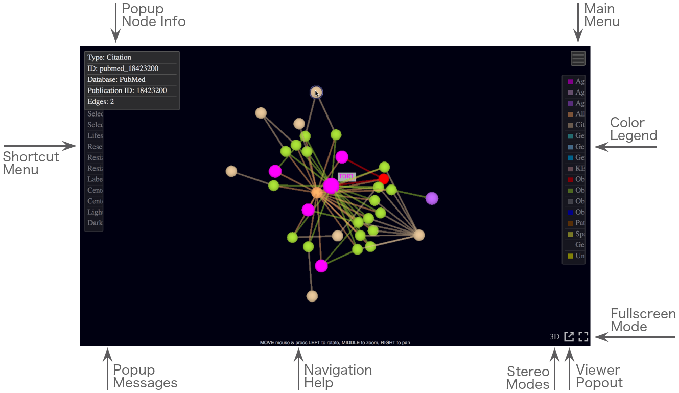 JANet Viewer Interface.
Screenshot of the JANet Viewer interface with element annotations.
JANet Viewer Interface.
Screenshot of the JANet Viewer interface with element annotations.
The viewer is the core of JANet visualization. All networks are rendered and visualized in this tab.
Use the mouse to rotate, zoom, pan, center on a node, and to toggle node selection and visibility.
Several control regions, annotated in the screenshot shown above, are activated either by hovering them with the mouse cursor or by clicking them:
- The Main Menu icon at the top right opens up the main viewer menu, offering a wide variety of options for exploring the network data and customizing the network view. At the top of the menu the total and currently selected number of nodes and edges are shown.
- The partially visible Color Legend at the right side becomes fully visible by hovering. It shows the current color code for all available node types and subtypes.
Clicking any subtype name will toggle the visibility of all nodes of the same type.
- The partially hidden Shortcut Menu at the left side becomes fully visible by hovering. It offers quick access to some frequently used options from the main menu, centering options and two viewer themes.
- The three icons at the bottom right activate special modes if they are clicked: a fullscreen mode, copying the viewer tab into a new browser tab/window and two side-by-side stereo modes.
By hovering a node, a popup window at the top left shows information about this node. By hovering some menu items, a popup window at the bottom left shows help information. It also pops up to show error and status messages.
The viewer popout copies the current network into a new browser tab or window. Be aware that the new view is build from scratch with default settings, including the generation of a network layout.
Info
Some statistics for AgeFactDB and JANet are shown here.
How to contact us.
Help
This documentation.
Network Definition
JANet offers two fundamentally different ways to define a network for visualization.
For the first way the network components and component types are selected first and then the network is generated according to built-in rules. This is how the tabs described above are working. Ageing factors are used as starting points, defining the network components in combination with the selected options.
As an example it is shown here how to build the direct neighbourhood network of the gene RAS2 from Saccharomyces cerevisiae, augmented with allele type and citation nodes.
Select the following options in the Ageing Factor Networks tab and click the Visualize button:
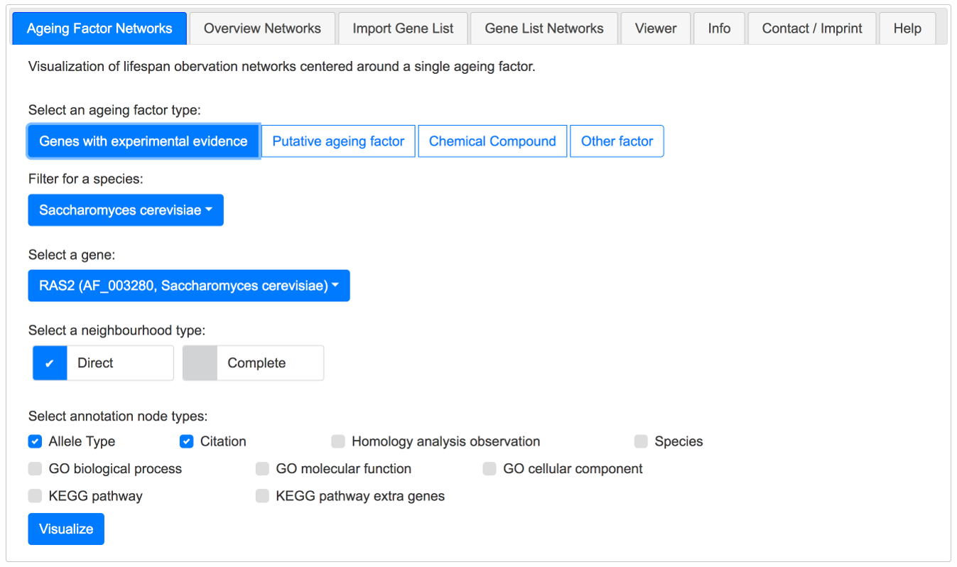 Example - Build the direct neighbourhood network ofRAS2 S. cerevisiae, augmented with allele types and citations.
The second way works inversely. It starts from the full network and then everything is removed that should not be part of the network. Any network components can be used to define a network in this way.
As an example it is shown here how to build a network containing all observations from the publication with the PubMed ID 12586694, augmented with allele type nodes.
The first step is done in the Overview Networks tab by selecting the following options and clicking the Visualize button:
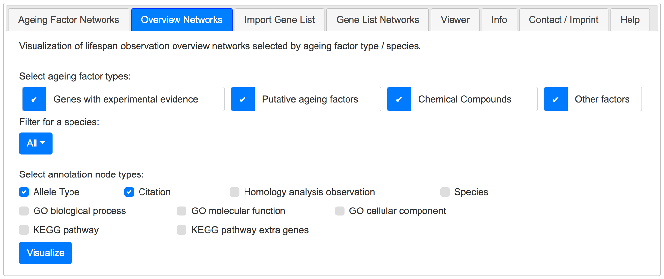 Example - Build the network of the publication with the PubMed ID 12586694, augmented with allele types - Part 1.
The next steps are done in the Viewer tab, where different node filters are applied sequentially to define the nodes to be removed:
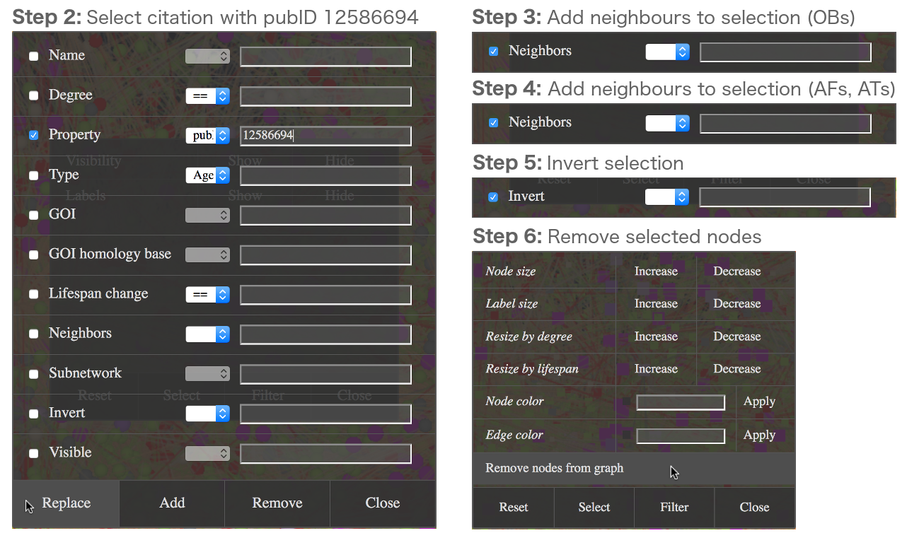 Example - Build the network of the publication with the PubMed ID 12586694, augmented with allele types - Part 2.
Viewer Options
Tabular View
A tabular view of the node information can be opened from the main menu (Show Tables).
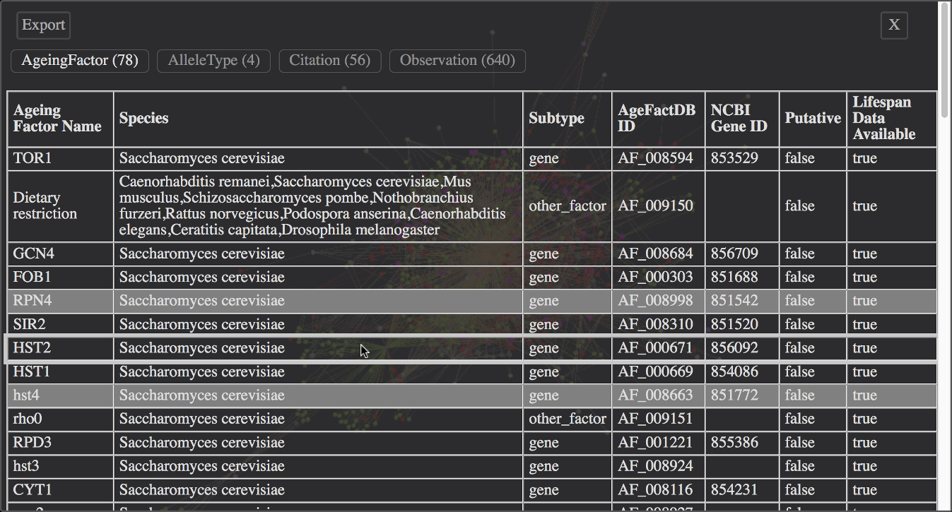 Example - Tabular view of the complete neighbourhood network of TOR1 from S.cerevisiae.
For each available node type a separate table exists. The node type can be selected by clicking the corresponding button at the top, displaying the node count in brackets (see example view above).
Currently selected nodes are marked in the table by a different row background color. Clicking a table row toggles the selection of it's node in the graph.
Clicking the table header toggles the selection of all nodes of the current type. The selection of nodes from other types remains unchanged.
The table data can be exported by clicking the Export button at the top left. For details please look at the Export section below.
Export
JANet offers three different types of export in the main menu (Export submenu).
Graph Image Export
The current view of the graph can be exported as an image in PNG format (Portable Network Graphics). The size of the image can be set independantly from the viewer size. This enables the export of high resolution images for publications.
The aspect ratio of the graph is kept during rescaling of the view.
Graph TSV Export
The graph can also be exported in TSV format (Tab-Separated Values) as node ID pairs defining the edges of the graph. This enables for example the import into many other network visualization and analysis tools.
Table Export
The node information tables can be exported in several formats: Microsoft Excel, CSV (Comma-Separated Values) and plain text.
A tabular view is opened like the one described in the section Tabular View above. The only difference is that the tables contain only the information from the currently visible nodes instead of all nodes. Information from hidden nodes is excluded. After clicking the Export button at the top right a new row with buttons for the different export formats appears, maybe with a delay for large networks.
Color Customization
JANet offers several options to customize colors.
Node Colors
The colors for all node types and subtypes, and also the background color of the viewer, can be customized within a dialog opened from the main menu (Change Colors).
They can be defined by different notations, according to the recommendations for CSS color specification. The most common notations are:
- A name from the list of named CSS colors, e.g.: green, lightskyblue
- A decimal RGB value triplett, e.g.: rgb(120, 100, 80)
- A decimal RGB value triplett extended by an alpha value for setting the translucency, e.g.: rgba(120, 100, 80, 0.5)
- A hexadecimal code, e.g.: #9ACD32
The alpha value ranges from 0 (full translucency) to 1 (opaque).
Additionally, the color of the currently selected nodes and edges can be set individually, described in the Node Manipulation section below.
Color Transfer
In the Visualization Techniques section of the introduction above there is described a data transfer technique. In JANet it is implemented for the data transfer from lifespan observations
to ageing factors. The direction of the lifespan change from all linked obervations (increased, decreased, unchanged) is combined into a color code for the ageing factor node:
| | opaque green | 100% observations with increased lifespan |
|---|
| | translucent green | ≥80% and <100% observations with increased lifespan |
|---|
| | opaque red | 100% observations with decreased lifespan |
|---|
| | translucent red | ≥80% and <100% observations with decreased lifespan |
|---|
| | opaque grey | 100% observations with unchanged lifespan |
|---|
| | translucent grey | ≥80% and <100% observations with unchanged lifespan |
|---|
| | orange | <80% observations of each direction |
|---|
The data transfer and color coding can be started from the shortcut menu at the left side (Lifespan Change to Ageing Factors). The ageing factor colors can also be set back to the default color from this menu (Reset Ageing Factor Colors).
If you delete lifespan observation nodes afterwards, the color is not adapted immediately for the ageing factor nodes connected to the deleted nodes. This enables to keep the transferred information from the deleted nodes until starting the transfer again.
Color Themes
There are two color themes available for the viewer tab: dark mode and light mode.
The default dark mode is optimized for a black background color of the viewer. The light mode is optimized for a white background color, helpful for example for the generation of views for printing.
It can be switched between these themes in the short cut menu at the left side (Light mode, Dark Mode).
Node Selection
Node selection is an essential part of the workflow in the JANet viewer. Many functions act specifically on the currently selected nodes, for example changing the node size and toggling the visibility of nodes and labels.
Selected nodes are marked by a different shape: cuboid instead of sphere.
There are four different ways to select/unselect nodes:
- With the mouse in the graph
- With the mouse in the info tables
- By filter rules
- By shortcut menu entries
Mouse Selection
The selection of individual nodes can be toggled by clicking a node in the graph with the left (main) mouse button.
Alternatively, it can also be toggled by clicking a data row in a node info table. Clicking the header row adds or removes all nodes of the corresponding type from
the current selection. See also the figure in the Tabular View section above.
Node Filter
The current selection can also be changed by defining and applying filter rules in the node filter dialog, available from the main menu in the Select Nodes and Manipulate Selected Nodes dialogs (Filter button):
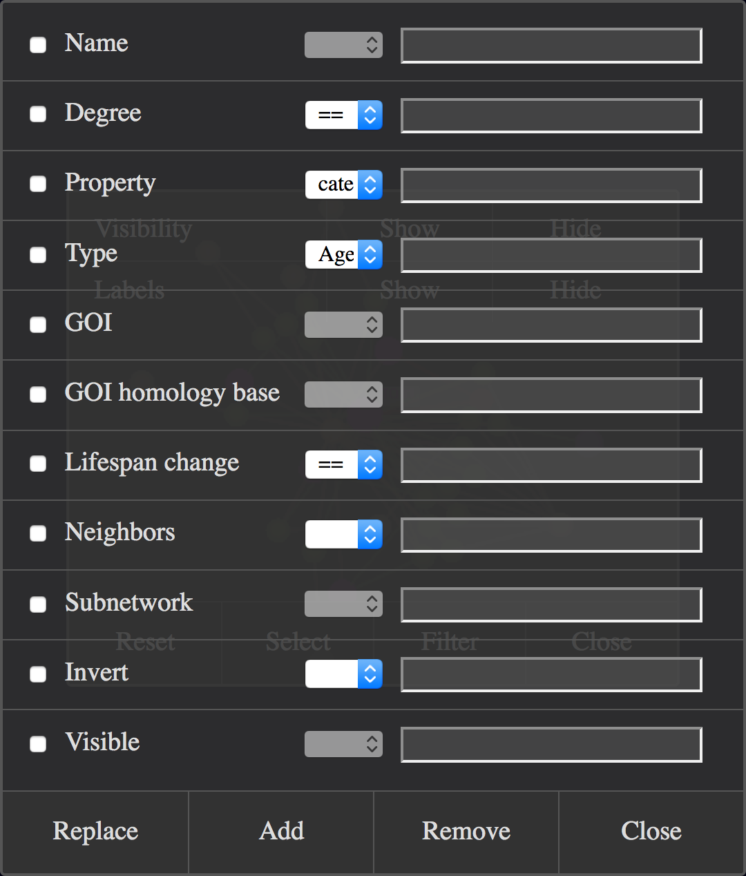 Node Filter Dialog Window.
A filter rule is defined by activating one or more of the predefined components (with the checkboxes at the left side) and setting the parameters.
Parameters can be a predefined value from a dropdown list, a value entered into a text input field, or a combination of both.
The components are usually combined using the boolean operator and. If for example one component would be Degree>5 and the other would be Type=AgeingFactor , then all ageing factor nodes with more than five edges would match the rule.
An exception are the components Neighbours and Subnetwork, where the matching nodes are added to those matching the other activated components.
And if no other components are activated, the base for defining matching nodes are the currently selected nodes.
Another exception are the Invert and Visible components, which cannot be combined with other components.
The rule is applied by clicking one of three buttons at the bottom of the dialog. Replace exchanges the currently selected nodes with the matching nodes.
Add merges the currently selected nodes with the matching nodes. Remove subtracts the matching nodes from the currently selected nodes.
The Filter dialog enables already complex filter rules. Even more complex selection strategies can be realized by applying multiple filter rules sequentially.
See part 2 of the example in the Network Definition section above.
Shortcut Menu Selection
The shortcut menu at the left viewer side offers also some node selection options:
All nodes can be selected or unselected, ageing factors and observations can be added to the current selection, and all labelled nodes can be selected.
Node Visibility
JANet offers three different ways to change the visibility of nodes:
- Toggle selected nodes
- Toggle by node type
- Toggle with the mouse
If a node is hidden, all edges of it are also hidden.
Toggle the Visibility of Selected Nodes
The Select dialog, available from the main menu (Select) has Show/Hide buttons that change the visibilty of the currently selected nodes.
Toggle the Visibility by Node Type
The color legend window at the right viewer side can also be used to change the visibility of specific node types by clicking a corresponding entry with the left (main) mouse button.
Hidden node types are indicated in the color legend by hiding the color square at the front.
This is a global switch that overrides the visibility switch in the Select dialog and switching with the mouse. This means that only if a node type is switched on in the color legend, the visibility can be changed using the Select dialog or the mouse.
Toggle the Visibility with the Mouse
The visibility of nodes can also be changed using the mouse.
In some cases the network topology is used to define which nodes are shown and which nodes are hidden if you click at a node.
There are two different modes available, selected by specific modifier keys, that define which neighbours of the clicked node are shown.
Independant of the network topology there can also be defined a screen region by dragging the mouse. All nodes outside of this region, indicated by a filled rectangle, are hidden. If an empty region is defined, all nodes are shown.
Please be aware that nodes of a type hidden globally, using the color legend, will stay hidden.
| Mouse Modes | Mouse Action | Visibility Action |
|---|
| Visibility | LEFT-CLICK | Show the clicked node and all direct neighbours (path depth = 1), hide all other nodes.
If nodes were already hidden by clicking a node, show all nodes. |
| Default, Label | ALT/OPTION LEFT-CLICK | Show the clicked node and all direct neighbours (path depth = 1), hide all other nodes.
If nodes were already hidden by clicking a node, show all nodes. |
| Default, Label, Visibility | SHIFT LEFT-CLICK | Show the clicked node, all direct neighbours and their direct neighbours (path depth = 2), hide all other nodes. |
| Default, Label, Visibility | SHIFT LEFT-CLICK + DRAG | Define a region, marked by a filled square; show nodes within the region, hide all other nodes.
If the region is empty, show all nodes. |
This option enables for example to explore quickly subnetworks of large complete neighbourhood and overview networks.
Node Labels
Each node has a predefined label that is initially hidden for most nodes. It usually consists of the node ID or node name. For lifespan observations it is the lifespan change value instead.
The display of node labels can be toggled in two ways:
- In the Select dialog, available from the the main menu (Select), the labels of all selected nodes can be switched on or off.
- Clicking a node in the mouse mode Label switches the label of this node on or off.
Besides, the shortcut menu at the left viewer side offers a quick way to show the label of all observations (Label Observations) and to select all nodes with a displayed label (Select labeled nodes (only))
Node Manipulation
The Main menu provides a node manipulation dialog (Manipulate selected Nodes). It offers to remove nodes from the network, to change the node size and color,
the node label size, and the edge color:
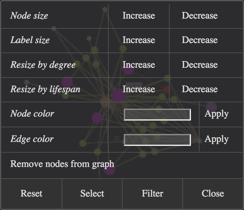 Manipulate Selected Nodes Dialog Window.
All manipulations are made on the currently selected nodes. For convenience, the dialog also offers the Select and Filter options from the Select Nodes dialog to redefine the current selection.
Initially, each node has a type-specific default size, with a few exceptions. The size can be changed individually or systematically to map quantitative data: lifespan change or degree (number of edges).
The size change by mapping quantitative data is also available from the Shortcut menu.
Set Node Size and Node Label Size Individually
Clicking the Increase button in the Node size row of the dialog increases the current radius of the selected nodes by a predefined factor. The radius is decreased by the same factor after clicking the Decreased button.
The node size is reset to the default size by clicking the Node size button.
Similarly, the node label size can be increased by clicking the Increase button in the Label size row of the dialog and decreased by clicking the Decreased button.
The node label size is reset to the default size by clicking the Label size button.
Set Node Size by Degree
The number of edges of a node is called degree. The minimum and maximum degree of nodes from the whole network are used to define the size range used for mapping the degree data.
Initially, there are defined a minimum and maximum node radius. If you use the option Resize Selected Nodes by Degree from the Shortcut menu, the minimum and maximum degrees are assigned to these size limits. Then the degree of the selected nodes is normalized to define the mapped radius within these limits.
Clicking the Increase button in the Resize by degree row of the dialog increases the maximum radius, while the minimum radius stays fixed. This expands the scale and increases the resolution. Similarly, clicking the Decrease button decreases the maximum radius and reduces the scale.
Please be aware that the node size does not reflect the degree directly. Instead, the node size difference between nodes reflects their degree difference.
If you want to increase the minimum radius, you can use the Increase button from the Node size row after you finished defining the size scale. This will shift also the size of larger nodes, keeping the size difference factors constant. But to prevent inconsistencies, you must apply all changes always identically to all nodes whose size should reflect their degree.
If nodes are deleted afterwards, the size is of nodes connected to the deleted nodes is not adapted immediately. Size changes must be initiated manually to reflect the modified network connectivity.
The node size is reset to the default size by clicking the Resize by degree button.
Set Node Size by Lifespan Change
The size of lifespan observation nodes can be set according to their lifespan change value as absolute value. The direction of the change is ignored because it is a stronger effect to decrease the lifespan by 200% than to increase it by 20%.
Similarly, the size of ageing factor nodes can be set according to their maximum lifespan change value as absolute value. Since other node types don't have a lifespan change value, their size will just be reset to their default size.
The minimum and maximum lifespan change of nodes from the whole network are used to define the size range used for mapping the lifespan change data.
Initially, there are defined a minimum and maximum node radius. If you use the option Resize Selected Nodes by Lifespan from the Shortcut menu, the minimum and maximum lifespan change values are assigned to these size limits. Then the lifespan change value of the selected nodes is normalized to define the mapped radius within these limits.
Clicking the Increase button in the Resize by lifespan row of the dialog increases the maximum radius, while the minimum radius stays fixed. This expands the scale and increases the resolution. Similarly, clicking the Decrease button decreases the maximum radius and reduces the scale.
Please be aware that the node size does not reflect the lifespan change value directly. Instead, the node size difference between nodes reflects their lifespan change value difference.
If you want to increase the minimum radius, you can use the Increase button from the Node size row after you finished defining the size scale. This will shift also the size of larger nodes, keeping the size difference factors constant. But to prevent inconsistencies, you must apply all changes always identically to all nodes whose size should reflect their lifespan change value.
If nodes are deleted afterwards, the size is of nodes connected to the deleted nodes is not adapted immediately. Size changes must be initiated manually to reflect the modified network connectivity.
The node size is reset to the default size by clicking the Resize by lifespan button.
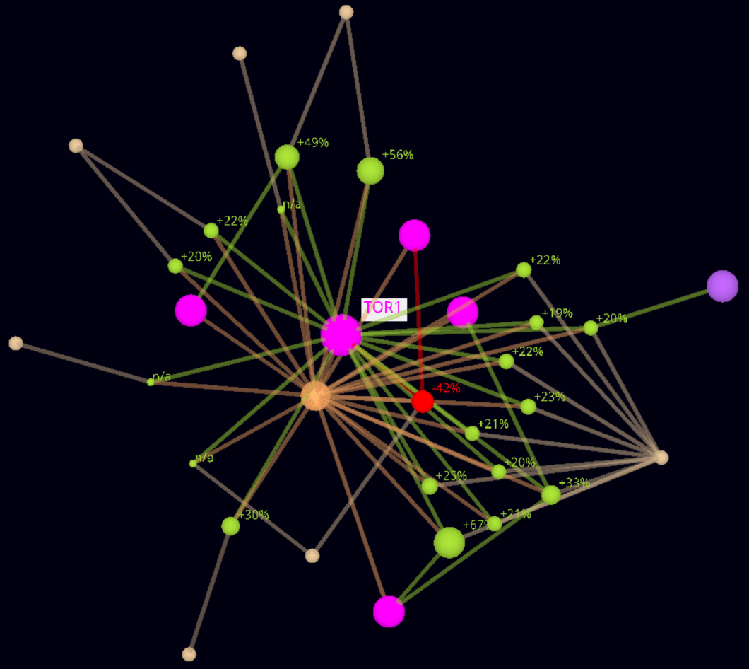 Example - Lifespan Observation Nodes Resized by Lifespan Change Value.
Direct neighborhood network of TOR1 S. cerevisiae, augmented with allele types and citations. Lifespan observation node sizes are changed proprtionally to the lifespan change.
For comparison, the nodes are also labeled with the lifespan change value.
Set Node Color Individually
The color of individual nodes can be set independant of their type and subtype by entering a color value in the Node color row of the dialog and clicking the Apply button.
Valid color values are the same as described in the Color Customization section above. As soon as a valid value was entered, a small square with the corresponding color is shown in front of the input field as indicator.
The node color is reset to the type/subtype-specific color by clicking the Node color button.
Set Edge Color Individually
The color of individual edges can be set independant of the color of their nodes by entering a color value in the Edge color row of the dialog and clicking the Apply button.
Valid color values are the same as described in the Color Customization section above. As soon as a valid value was entered, a small square with the corresponding color is shown in front of the input field as indicator.
An edge is selected by selecting both nodes which define the edge.
The edge color is reset to the type/subtype-specific color by clicking the Edge color button.
Remove Nodes
Clicking the Remove nodes from graph button will delete the selected nodes and their edges from the network.
It will also trigger an adaptation of the network layout. And if lifespan observation nodes were deleted, the maximum lifespan change value of ageing factors will be recalculated.
Reset Node Manipulations
Clicking the global Reset button at the bottom left will undelete all deleted nodes and set node size, label size and label color to the default value.
It will also trigger an adaptation of the network layout. And if lifespan observation nodes were undeleted, the initial maximum lifespan change value of ageing factors will be restored.
Network Layout Generation
The network layout generation can be controlled using the Layout submenu within the main menu:
The submenu offers the choice between the three layout algorithms described in the Network Layout Algorithms section of the introduction:
- D3 (3D-forced)
- FR (Fruchterman-Reingold)
- FMMM (Fast Multipole Multilevel Method)
The algorithms have the following characteristics:
|
D3 |
FR |
FMMM |
Comment |
| Network Size |
medium, up to several hundred nodes |
small, up to about hundred nodes |
large, up to many thousand nodes |
There are no actual size restrictions. This are just recommendations for obtaining better layouts. |
| Speed |
fast |
fast |
slow |
Although the FMMM layout generation is much slower, it usually provides better layouts for medium to large networks. |
| Processing Location |
locally, in your browser |
locally, in your browser |
remotely, on the JANet server |
The FMMM layout is calculated remotely by a modified version of the Java program BiolayoutExpress 3D to speed up the layout generation and make the speed independant of the power of your computer. |
| Layout Cache |
no |
no |
yes |
FMMM layouts may take several minutes or longer and are therefore cached remotely on the JANet server. So the layouts are available nearly instantly if requested again by any user. |
| Display of Intermediate Layouts |
yes |
yes |
no |
The layout generation is an iterative process of refining the node positions. The result of each refinement step is displayed for the layouts processed locally. |
| Stoppable Layout Generation |
yes |
yes |
no |
The layout generation/refinement process can be disrupted from the layout submenu of the main menu (Stop D3/FR). |
| Layout Refinement |
yes |
yes |
no |
The layout can be refined by starting additonal layout calculation steps from the layout submenu of the main menu (Update D3/FR). The number of refinement steps can be set also within this menu. |
| Reproducible Layout |
yes |
yes |
yes |
The layout generated for a specific network by a specific algorithm, with the same number of refinement steps, will always be the same. |
Known Problems
The FMMM layout generation might run into a timeout error. This only means that the connection between the JANet server and your browser was disrupted. It usually doesn't mean that the layout generation was disrupted. The layout will most probably be finished and cached on the server. So you should wait a while and then try again. If caching was succesful, the cached layout will be applied directly. Otherwise you should wait longer before you try it again.
Mouse Control
The interactive features of the viewer are mainly controlled by using the mouse pointer.
Mouse Modes
You can choose between three mouse modes in the main menu:
The Default mode is designed as general purpose mode. The other modes replace some options for special purposes.
The Label mode enables to toggle node labels quickly.
The Visibility mode enables to toggle the visibility of subnetworks also on systems where some of the modifier key combinations of the Default mode don't work.
Mouse Actions
This section summarizes the mouse actions available in the graphics area of the viewer. To simplify the description of the mouse actions, the modifier key and mouse button synonyms were reduced to a single unified name and defined separately, together with other mouse-related nomenclature.
| Mouse Modes |
Mouse Actions |
Location |
Viewer Action |
| Default |
LEFT-CLICK |
node |
Toggle the selection of the clicked node. |
| Label |
LEFT-CLICK |
node |
Toggle the label visibility of the clicked node. |
| Visibility |
LEFT-CLICK |
node |
Show the clicked node and all direct neighbours (path depth = 1), hide all other nodes. If nodes were already hidden by clicking a node, show all nodes. |
| Default, Label, Visibility |
LEFT-CLICK + DRAG |
anywhere |
Rotate the network around the current center. |
| Default, Label, Visibility |
WHEEL-UP,
MIDDLE-CLICK + DRAG up |
anywhere |
Zoom in. |
| Default, Label, Visibility |
WHEEL-DOWN,
MIDDLE-CLICK + DRAG down |
anywhere |
Zoom out. |
| Default, Label, Visibility |
RIGHT-CLICK + DRAG |
anywhere |
Move the network along the X-axis or Y-axis, according to the mouse movement. |
| Default, Label, Visibility |
CTRL LEFT-CLICK,
CMD LEFT-CLICK |
node |
Set the rotation center to the clicked node and move it to the viewer center. |
| Default, Label, Visibility |
SHIFT LEFT-CLICK |
node |
Show the clicked node, all direct neighbours and their direct neighbours (path depth = 2), hide all other nodes. |
| Default, Label, Visibility |
SHIFT LEFT-CLICK + DRAG |
node |
Define a region, marked by a filled square; show nodes within the region, hide all other nodes. If the region is empty, show all nodes. |
| Default, Label |
ALT LEFT-CLICK |
node |
Show the clicked node and all direct neighbours (path depth = 1), hide all other nodes. If nodes were already hidden by clicking a node, show all nodes. |
| Unified Name |
Type |
Synonyms |
| LEFT |
mouse button |
main, primary |
| RIGHT |
mouse button |
secondary |
| MIDDLE |
mouse button |
third, wheel button |
| SHIFT |
modifier key |
|
| CMD |
modifier key |
command |
| CTRL |
modifier key |
Strg, control |
| ALT |
modifier key |
alternate, option |
| CLICK |
movement |
Move a button down (press) and up (release) within a short time period. |
| DOUBLE-CLICK |
movement |
Move a button down (press) and up (release) two times within a short time period. |
| DRAG |
movement |
Move the mouse while a button is pressed. |
| WHEEL-UP |
movement |
Rotate the scroll wheel upwards (away from the hand). |
| WHEEL-DOWN |
movement |
Rotate the scroll wheel downwards (towards the hand). |
Freeze / Unfreeze Graph
JANet uses the hardware-accelerated graphics library WebGL to display and animate the network graphics. This has many advantages but also a disadvantage: the network graphics is always updated about 30 times per second, even if nothing changes. This leads to a constant high CPU usage and significant energy consumption.
The main menu offers manual control of the update process. You can stop further updates (Freeze Graph) and reduce the CPU usage and energy consumption. And you can restart updating (Unfreeze Graph) if you want to resume working with JANet.
Another way to stop the update process is to switch to another browser tab in the same browser window. It is not sufficient to switch to another window while the JANet tab remains the active tab in it's window.. And it is also not sufficient to switch to another tab inside JANet.